Load profiles¶

CLOVER has the functionality to build load profiles from the bottom-up, summarised in the following steps:

Input the devices or appliances available in the community
Input the usage profile of each device throughout the day and year
Calculate the number of devices in use throughout the lifetime of the system
Calculate the daily utilisation profile of each device
Calculate the number of devices in use in every hour
Calculate the load profile of each device
Calculate the total load profile of the community.

This process is performed by the Load module, described in this section. The terms device and appliance are used interchangeably, meaning any piece of equipment that uses electricity, and specific meanings of other similar terms (for example usage and utilisation) will be made explicit where relevant.

Preparation¶

Input the devices in the community¶

CLOVER allows the user to include as many devices as desired in their load profile. These are input using the Devices input CSV in the Load folder for the given location, which can be edited directly. Let’s look at the devices included for Bahraich:

	Device	Available	Power	Initial	Final	Innovation	Imitation	Type
0	light	Y	3	2.00	4.00	0.04	0.50	Domestic
1	phone	Y	5	2.20	3.00	0.02	0.20	Domestic
2	radio	Y	10	0.28	0.35	0.01	0.20	Domestic
3	tv	Y	20	0.08	0.90	0.03	0.25	Domestic
4	laptop	Y	40	0.01	0.50	0.02	0.10	Domestic
5	fridge	Y	50	0.00	0.50	0.02	0.20	Domestic
6	fan	Y	10	0.10	2.00	0.04	0.30	Domestic
7	kerosene	Y	1	3.40	2.00	0.02	0.10	Domestic
8	mill	Y	750	0.01	0.10	0.02	0.20	Commercial
9	workshop	Y	350	0.05	0.05	0.02	0.20	Commercial
10	SME	Y	200	0.05	0.03	0.25	0.25	Commercial
11	streetlight	Y	25	0.20	0.20	0.00	0.00	Public

This CSV contains many variables, some of which are more obvious than others, summarised in the table below:

Variable	Explanation
`Device`	Unique name of the device
`Available`	Device is included (`Y`) or not (`N`) in the community load
`Power`	Device power consumption (W)
`Initial`	Average ownership of the device per household at the start of the time period
`Final`	Average ownership of the device per household at the end of the time period
`Innovation`	Parameter governing new households acquiring device
`Imitation`	Parameter governing households copying others
`Type`	Classification of the device as a `Domestic`, `Commercial` or `Public` device

Take the example of the device light, which represents an LED bulb. It is available in the load profile (Available = Y), has a power rating of 3 W, and classified as a Domestic load. At the start of the simulation period there is an average two LED bulbs per household (Initial = 2.00) which, over time, increases to four bulbs per household (Final = 4.00) by the end of the considered time period - which we defined to be to 20 years in the General Setup section.

The two remaining variables describe how quickly the average ownership per household increases: to generalise, Innovation describes how likely a household is to get a new appliance based on how much they like new things and Imitation describes how much a household is influenced by others already having the device. These are inputs into a model of how quickly devices diffuse throughout the community (described in more detail later) but, simply put, the larger these numbers the quicker households will acquire them. These should be treated almost as qualitative measures: the values for a more desirable appliance like a television should be higher than (for example) a radio. You can use later outputs from the Load module to check that your appliance diffusion seems viable.

If you do not want to include any demand growth over time by keeping the number of appliances the same throughout the simulation, it is possible to turn off this feature simply by setting the values for Initial and Final to be the same, which will negate the Innovation and Imitation parameters (for example streetlight does this). Bear in mind that an increase in the number of households, defined when establishing the location, will result in an increase in the number of devices as the latter is calculated on the basis of the number of devices per household.

One of the devices, kerosene, is different from the others and is the only device which must remain present in the Devices file. CLOVER has the functionality to account for the usage of backup non-electric lighting devices, such as kerosene lamps, which are used during periods when electricity is unavailable. This is useful when investigating electricity systems with less than 100% reliability, for example. This device is therefore necessary as an input for later functions and must be present here, and have corresponding utilisation profiles, described later. If backup sources of non-electric lighting are not relevant to your investigation, set Initial = 0 and Final = 0 in the Devices file to not consider it whilst still allowing the other functions to operate as expected. If a different non-electric lighting source is relevant, such as candles, complete the input data for that source but the name must remain as kerosene in the Devices file.

With this in mind, complete the Devices input CSV for your investigation.

Input the device utilisation profiles¶

CLOVER first considers the service that appliances provide as a necessary step in understanding the electricity demand of the community, rather than jumping directly to the latter. This is because two devices may provide very similar services, and the times of using those devices may be very similar, but the electricity requirements could be very different: LED and incandescent light bulbs, for example. By considering the demand for the service as a first step it is possible to more easily consider issues such as the usage of efficient, low-power devices which are becoming more common.

The utilisation of a device is defined to be the probability that a device is being used, given that it is present in the community. Utilisation values can vary hourly (throughout the day) and monthly (throughout the year) and must be between 0 (the device is never used in a specific hour) to 1 (it is always used). Utilisation profiles for each device are found in the Device utilisation folder in the Load folder.

Every device listed in the Devices input CSV must have a utilisation profile associated with it for CLOVER to calculate the load demand correctly and be named [device]_times. Even if a device has Available = N in the Devices input CSV, CLOVER will still use the utilisation profile but not eventually include the load in the final total community demand. If you do not want to include a device at all it is much easier to delete its entry from the Devices input CSV.

Each utilisation profile is a 24 x 12 matrix of utilisation values, corresponding to the hour of the day for each month of the year. Let’s take a look at the example of light:

   1     2     3     4     5     6     7     8     9     10    11
 0.39  0.39  0.39  0.39  0.39  0.39  0.39  0.39  0.39  0.39  0.39  0.39
 0.39  0.39  0.39  0.39  0.39  0.39  0.39  0.39  0.39  0.39  0.39  0.39
 0.39  0.39  0.39  0.39  0.39  0.39  0.39  0.39  0.39  0.39  0.39  0.39
 0.39  0.39  0.39  0.39  0.39  0.39  0.39  0.39  0.39  0.39  0.39  0.39
 0.39  0.39  0.39  0.39  0.48  0.56  0.46  0.39  0.39  0.39  0.39  0.39
 0.39  0.39  0.47  0.48  0.23  0.12  0.28  0.45  0.53  0.57  0.40  0.39
 0.58  0.48  0.22  0.00  0.00  0.00  0.00  0.00  0.00  0.05  0.37  0.53
 0.00  0.00  0.00  0.00  0.00  0.00  0.00  0.00  0.00  0.00  0.00  0.00
 0.00  0.00  0.00  0.00  0.00  0.00  0.00  0.00  0.00  0.00  0.00  0.00
 0.00  0.00  0.00  0.00  0.00  0.00  0.00  0.00  0.00  0.00  0.00  0.00
0.00  0.00  0.00  0.00  0.00  0.00  0.00  0.00  0.00  0.00  0.00  0.00
0.00  0.00  0.00  0.00  0.00  0.00  0.00  0.00  0.00  0.00  0.00  0.00
0.00  0.00  0.00  0.00  0.00  0.00  0.00  0.00  0.00  0.00  0.00  0.00
0.00  0.00  0.00  0.00  0.00  0.00  0.00  0.00  0.00  0.00  0.00  0.00
0.00  0.00  0.00  0.00  0.00  0.00  0.00  0.00  0.00  0.00  0.00  0.00
0.00  0.00  0.00  0.00  0.00  0.00  0.00  0.00  0.00  0.00  0.00  0.00
0.00  0.00  0.00  0.00  0.00  0.00  0.00  0.00  0.00  0.00  0.00  0.00
0.47  0.08  0.00  0.00  0.00  0.00  0.00  0.00  0.00  0.39  0.74  0.76
0.93  0.93  0.54  0.51  0.23  0.03  0.00  0.26  0.79  0.93  0.93  0.93
0.93  0.93  0.93  0.93  0.93  0.93  0.90  0.93  0.93  0.93  0.93  0.93
0.93  0.93  0.93  0.93  0.93  0.93  0.93  0.93  0.93  0.93  0.93  0.93
0.93  0.93  0.93  0.93  0.93  0.93  0.93  0.93  0.93  0.93  0.93  0.93
0.88  0.88  0.88  0.88  0.88  0.88  0.88  0.88  0.88  0.88  0.88  0.88
0.83  0.83  0.83  0.83  0.83  0.83  0.83  0.83  0.83  0.83  0.83  0.83

This device, representing an LED bulb from before, has a changing utilisation profile throughout the day: it is never used during the middle of the day (utilisation is 0.00), is very likely to be used in the evenings (up to 0.93), and some lights in the community are likely to be left on overnight (0.39). The utilisation of this device also changes throughout the year: in January (month 0) the utilisation at 18:00 is 0.93, but is 0.00 in July (month 6), owing to the changing times of sunset.

Making a representative utilisation profile will depend significantly on the specifics of your own investigation. These could come from primary data collection (indeed, the utilisation profile shown above did) or from your best estimate of what the demand for service is likely to be. Bear in mind that the probability that a device being used is an average over the entire community, so this should represent the utilisation of an “average” household without considering inter-household variations. To model device utilisation as the same throughout the year, use the same 24-value column for each of the 12 months.

For every device you have listed in the Devices input CSV, complete a corresponding utilisation profile matrix and ensure that is is called [device]_times.

Building load profiles¶

Calculating the number of devices in the community¶

The next step is to know how many devices there are in the community at any given time which, when combined with the utilisation profiles, will then allow us to calculate how many are in use. This step is relatively straightforward in that it takes information we have already input (into the Devices CSV file) and calculates everything for us. It also accounts for the growing number of devices in the community, if we chose to use that.

To calculate this automatically for all of the devices listed, run the function

Load().number_of_devices_daily()

in the console. This will take every device listed and calculate the number in the community on every day of our 20 year investigation period, and save them as a CSV file in the Device ownership folder in the Load folder with title format of [device]_daily_ownership.csv. Let’s take a look at the light device again and look at the first and final number of devices in the community:

Initial light ownership = 200
Final light ownership = 487

The final light ownership perhaps looks higher than expected, but when we take into account how much the community has grown it makes sense:

The slight discrepancy in the two values likely comes from the diffusion model tending towards (but never quite reaching) the final value of average ownership and/or rounding errors.

Calculating the daily utilisation profiles¶

The utilisation profiles input for each device was defined by month but, if we assigned that utilisation profile for the whole month-long period, there would be a sharp transition between each month which would be unrealistic. To overcome this CLOVER interpolates between the monthly values to give a smooth transition between every day, meaning that there are no harsh boundaries where demand suddenly changes. This process is also performed automatically by CLOVER. Run the following function in the console to calculate this:

Load().get_device_daily_profile()

This function takes the (monthly) utilisation inputs and converts them to a daily utilisation input of size 365 x 24 and saves it in the Device utilisation folder in the Load folder using the title format [device]_daily_times.csv. CLOVER assumes that the values stated in the monthly utilisation profile apply to the middle day of each month when interpolating to the daily scale.

As an example, let’s compare the monthly input values for January and February against the first week of daily values for the light device:

Input values for January and February:

     Jan   Feb
 0.39  0.39
 0.39  0.39
 0.39  0.39
 0.39  0.39
 0.39  0.39
 0.39  0.39
 0.58  0.48
 0.00  0.00
 0.00  0.00
 0.00  0.00
0.00  0.00
0.00  0.00
0.00  0.00
0.00  0.00
0.00  0.00
0.00  0.00
0.00  0.00
0.47  0.08
0.93  0.93
0.93  0.93
0.93  0.93
0.93  0.93
0.88  0.88
0.83  0.83

Daily varying values:

        0      1      2      3      4      5      6
 0.390  0.390  0.390  0.390  0.390  0.390  0.390
 0.390  0.390  0.390  0.390  0.390  0.390  0.390
 0.390  0.390  0.390  0.390  0.390  0.390  0.390
 0.390  0.390  0.390  0.390  0.390  0.390  0.390
 0.390  0.390  0.390  0.390  0.390  0.390  0.390
 0.390  0.390  0.390  0.390  0.390  0.390  0.390
 0.555  0.557  0.559  0.560  0.562  0.564  0.566
 0.000  0.000  0.000  0.000  0.000  0.000  0.000
 0.000  0.000  0.000  0.000  0.000  0.000  0.000
 0.000  0.000  0.000  0.000  0.000  0.000  0.000
0.000  0.000  0.000  0.000  0.000  0.000  0.000
0.000  0.000  0.000  0.000  0.000  0.000  0.000
0.000  0.000  0.000  0.000  0.000  0.000  0.000
0.000  0.000  0.000  0.000  0.000  0.000  0.000
0.000  0.000  0.000  0.000  0.000  0.000  0.000
0.000  0.000  0.000  0.000  0.000  0.000  0.000
0.000  0.000  0.000  0.000  0.000  0.000  0.000
0.615  0.605  0.594  0.584  0.574  0.563  0.553
0.930  0.930  0.930  0.930  0.930  0.930  0.930
0.930  0.930  0.930  0.930  0.930  0.930  0.930
0.930  0.930  0.930  0.930  0.930  0.930  0.930
0.930  0.930  0.930  0.930  0.930  0.930  0.930
0.880  0.880  0.880  0.880  0.880  0.880  0.880
0.830  0.830  0.830  0.830  0.830  0.830  0.830

Note that the daily utilisation CSV file has a slightly different structure (days are presented as rows) but we have transposed it here and rounded to three decimal places for comparability and readability. The hours where there is a difference between utilisation in January and February (hours 6 and 17) also vary in the daily profile, whilst the others remain the same as expected. As mentioned above, note that the utilisation input for January is not the same as the daily utilisation on day 0: the former is assumed to be for the middle day of the month in January, whereas the latter is halfway between the inputs for December and January. We can check this:

December utilisation at 6:00: 0.53
January utilisation at 6:00: 0.58
Midpoint utilisation between December and January: 0.555
Day 0 utilisation at 6:00: 0.555

As expected, the two values match.

Calculating the number of devices in use¶

Now that we have both the number of devices in the community on a given day, and the daily utilisation profile of each device, we can calculate the number of devices that are in use at any given time. CLOVER does this automatically for each type of device by using a binomial random number generator: the number of trials is the number of devices, and the probability is the utilisation value for that hour. To do this, run the following function in the console:

Load().devices_in_use_hourly()

This function will take a while to complete as it runs through each type of device and randomly assigns the number in use over the full 20 year period, and needs to be performed once only. The outputs are saved as CSV files in the Devices in use folder in the Load folder, using the title format [device]_in_use.csv, so that they can be used as consistent inputs when used by CLOVER. Note that rerunning this function will create a new profile which will differ every time because of the random statistics used to generate it: if you need to rerun this function but want to keep your previous files, save a copy of them elsewhere otherwise they will be overwritten.

Let’s consider the light device over the first three days of its usage:

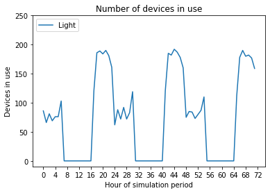
The number of light devices in use in a given hour changes throughout the day: as expected from the utilisation profile, some are in use overnight, none are in use during the day, and most are in use in the evenings. Comparing between days, the number of devices in use in a certain hour also varies.

Calculating the load profile of each device¶

Now that we know the number of each device in use at any given time, and the power rating of each from the Device input CSV, it is straightforward to get the load profile of each device. Run the following function in the terminal:

Load().device_load_hourly()

This function uses the [device]_in_use.csv file and the power rating to save a new CSV file in the Device Load folder in the Load folder using the title format [device]_load.csv.

Let’s now compare two devices, light and tv, to see how the number in use and load demand vary over the first three days:

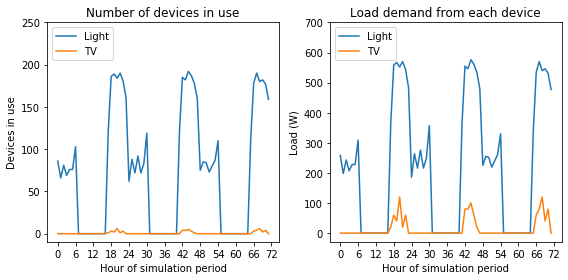
Comparing the two devices, the usage of tv devices is limited to the evening periods only and very few are ever in use, owing to the low average ownership. When we compare the load demanded by each device, tv has a more significant effect, albeit still relatively small, as the relative power rating is higher than that of light.

Calculating the total load demand of the community¶

Knowing the electricity demand of each appliance allows us to combine these to give the total electricity demand of the entire community over the duration of the investigation. Once again, CLOVER calculates this automatically when you run the following function in the console:

Load().total_load_hourly()

This function adds together all of the devices listed in the Device input file that have Available = Y and creates a new CSV in the Device load folder in the Load folder called total_load.csv. This also uses another of the input parameters from before, Type, to split the load into three categories: Domestic for households, Commercial for businesses and enterprises, and Public for community-level electricity uses.

With this, we now have the necessary load data to input into our simulations.

Troubleshooting¶

Most of the processes for generating load profile are automated but there are ample opportunities for simple mistakes when inputting the data which will cause errors. Solving the issues is normally simple but finding where they appear can be much harder, so if they come up:

Check that you have used consistent spelling and capitalisation for your devices throughout as these are case sensitive, e.g. radio and Radio will be treated as two completely different devices
Check that your file names correspond to the correct devices and are in the correct formats, e.g. radio has a utilisation profile named radio_times
Ensure that your input variables are in the correct format, for example Type is either Domestic, Commercial or Public
Ensure that your utilisation profiles are the correct size and format, and have the correct naming convention including the .csv suffix
Ensure that your device power is input in Watts (W), not kilowatts (kW)
Ensure that you have completed each of the steps in the correct order

Extension and visualisation¶

Using your own load profile¶

CLOVER gives users the functionality to construct their own load profiles from the bottom up, but sometimes you already have a load profile which you want to use directly without trying to recreate it using the Load module. This is straightforward to do, but your own load profile must be in the same format as the one generated by the Load module. To do this:

Ensure that your load profile is in the correct format: at an hourly resolution for the duration of your simulation period, measured in Watts (not kilowatts), and with the Domestic, Commercial and Public headings
Name your profile total_load.csv and copy it into the Device load folder in the Load folder of your location
Run the function Load().get_yearly_load_statistics('total_load.csv') to get the yearly load statistics
Copy kerosene_load.csv into the same folder (the values can be changed to zero, or the outputs ignored later, as necessary)

If you do not have Domestic, Commercial and Public loads, or they are combined into one category, it is most straightforward to include them all together in a single headed column (e.g. Domestic). The kerosene_load.csv needs to be included for compatibility with the later functionality, but the outputs relating to this can be ignored or the values in that profile can be set to zero for completeness. The Load().get_yearly_load_statistics('total_load.csv') is used later in the simulation process for sizing equipment (such as the inverters) so must be updated from the default case study values provided.

Comparing domestic, commercial and public electricity demand¶

Let’s take a look at how the three demand types compare over the first three days of the simulation period:

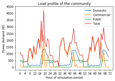
This allows us to compare the different types of demands in the community and how they vary throughout the day:

The Domestic demand is highest in the evening due to lighting and entertainment (such as TV) loads
The Commercial demand peaks in the day and has high variability caused by a smaller number of higher-power devices
The Public demand, composed here as streetlight only, has a consistent load profile as it is modelled to operate on a timed basis

Varying demand throughout the year¶

We can also see how these demands vary over the year by reformatting the data into daily demands. For visibility let’s look at a five-day rolling average, with the raw data plotted behind it:

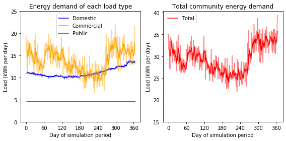
Note that the axes of the two subplots use the same scale but the axis of the right plot, showing the total community demand, is shifted upwards. Commercial demand, as before, displays the largest amount of variation both between days and over the course of the year, in this case because of varying agricultural demand. The Domestic demand has relatively little day-to-day variation but there is a noticeable decrease in the summer as lighting demand decreases. The growth in Domestic device ownership also results in the growth of the daily load demand (comparing January and December), almost exceeding the Commercial demand. Finally the Public demand remains the same throughout the year, as expected.

The total community demand is shown on the left. Its structure is mostly governed by the variation in the Commercial demand, but the effect of the Domestic demand can be seen when comparing the upwards shift in load comparing the start and end of this year-long profile.

Growing demand over the investigation period¶

We can see how load grows in the community across the investigation period, for example to replicate how appliance ownership might grow over time as a community develops economically. Let’s reformat the load data into yearly totals and compare them across the 20-year period:

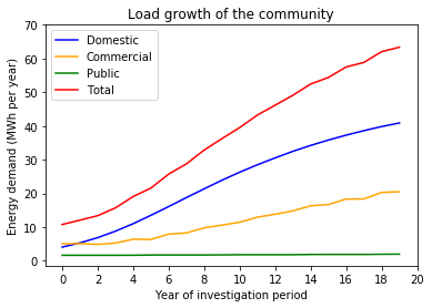
We can see here that the Domestic and Commercial loads both increase over time, but the Domestic increases much faster than Commercial and therefore is the greatest contributor to the total load soon after the first year (as we saw in earlier). The Public demand meanwhile remains the same throughout.