Electricity system simulation
Preparation
Now that we have completed both the electricity generation and demand inputs for our investigation we are almost ready to simulate an electricity system. This will allow us to model the technical performance of an electricity system of a given size and its ability to meet the load demanded by the community. At this stage we consider only the technical performance, rather than the financial or environmental considerations, which will come later when we optimise the sizing of the systems.
Before we can simulate a system we must first provide inputs for its technical performance and the conditions of the scenario under which we want it to operate.
Electricity system inputs
The inputs for the technical performance of the system are included in
the Energy system inputs file, which is located in the Simulation
folder of your location folder.
Let’s look at the inputs included for the Bahraich case study:
| 0 | 1 | 2 | |
|---|---|---|---|
| 0 | Battery maximum charge | 0.900 | State of charge (0.0-1.0) |
| 1 | Battery minimum charge | 0.400 | State of charge (0.0-1.0) |
| 2 | Battery leakage | 0.004 | Fractional leakage per hour |
| 3 | Battery conversion in | 0.950 | Conversion efficiency (0.0-1.0) |
| 4 | Battery conversion out | 0.950 | Conversion efficiency (0.0-1.0) |
| 5 | Battery cycle lifetime | 1500.000 | Expected number of cycles over lifetime |
| 6 | Battery lifetime loss | 0.400 | Fractional loss over lifetime (0.0-1.0) |
| 7 | Battery C rate discharging | 0.330 | Discharge rate |
| 8 | Battery C rate charging | 0.330 | Charge rate |
| 9 | Transmission efficiency DC | 0.950 | Efficiency of DC distribution network |
| 10 | Transmission efficiency AC | 0.950 | Efficiency of AC distribution network |
| 11 | DC to AC conversion | 0.950 | Conversion efficiency (0.0-1.0) |
| 12 | DC to DC conversion | 0.950 | Conversion efficiency (0.0-1.0) |
| 13 | AC to DC conversion | 0.800 | Conversion efficiency (0.0-1.0) |
| 14 | AC to AC conversion | 0.980 | Conversion efficiency (0.0-1.0) |
These variables control how the electricity system performs, in particular the performance of the battery storage and the conversion efficiencies in the system. The table below describes in more detail what each one means:
| Variable | Explanation |
|---|---|
Battery maximum charge |
Maximum permitted state of charge of the battery |
Battery minimum charge |
Minimum permitted state of charge of the battery |
Battery leakage |
Fraction of the energy stored in the battery lost per hour |
Battery conversion in |
Conversion efficiency of energy entering the battery |
Battery conversion out |
Conversion efficiency of energy leaving the battery |
Battery cycle lifetime |
Number of charging cycles expected from the battery over its lifetime |
Battery C rate discharging |
C-rate of the battery whilst providing energy |
Battery C rate charging |
C-rate of the battery whilst receiving energy |
Transmission efficiency DC |
Transmission efficiency of a DC distribution network |
Transmission efficiency AC |
Transmission efficiency of an AC distribution network |
DC to AC conversion |
Conversion efficiency from DC power to an AC distribution network |
DC to DC conversion |
Conversion efficiency from DC power to an DC distribution network |
AC to DC conversion |
Conversion efficiency from AC power to an DC distribution network |
AC to AC conversion |
Conversion efficiency from AC power to an AC distribution network |
The variables Battery maximum charge and Battery minimum charge
refer to the maximum and minimum permitted states of charge of the
battery: in this case the battery is allowed to cycle between 90% and
40% of its total capacity, resulting in a depth of discharge (DOD) of
50%, and meaning that 50% of the total installed battery capacity is
actually usable by the system. Battery leakage is the fraction of
energy that leaks out of the battery every hour, in this case 0.004
or 0.4% of the energy presently stored in it per hour.
Battery conversion in and Battery conversion out are the
conversion efficiencies of energy being supplied to and from the battery
respectively; when multiplied together these give the battery round-trip
efficiency.
Battery cycle lifetime refers to the number of charging and
discharging cycles that the battery can be expected to perform over its
lifetime, with the lifetime defined to be over when the battery has
degraded by Battery lifetime loss; in this case
Battery lifetime loss = 0.2 (as is typical for this definition) and
so the lifetime is over when the battery provides just 80% of its
original capacity. The battery degradation is calculated by multiplying
the lifetime loss by the energy throughput of the battery (at a given
point in time) and then dividing by the expected cumulative energy
throughput over the lifetime of the battery (the cycle lifetime
multiplied by the depth of discharge and total capacity). This
simplified method does not account for the effects of temperature or
reduced cycling which may affect the lifetime of a battery in practice.
Finally for the battery parameters, Battery C rate discharging and
Battery C rate charging are the C-rates for discharging and charging
the batteries, measured as the maximum permitted fraction of the battery
capacity that can be stored or supplied in one hour. These battery
parameters can be taken from a datasheet provided by a battery
manufacturer or used as indicative values in more general
investigations. They are also agnostic to the type of battery technology
being investigated, for example lead acid or lithium ion batteries. Some
of these parameters will be dependent on one another: for example, a
given battery being used with a higher DOD will likely have a lower
cycle lifetime. These relationships are often available on battery
datasheets (for example as performance curves) but need to be input
manually and individually here. Similarly, higher C-rates will also
likely result in lower cycle lifetimes.
Let’s take a look at some of the variables:
Maximum state of charge: 90%
Minimum state of charge: 40%
Depth of discharge: 50%

Battery input efficiency: 95%
Battery output efficiency: 95%
Round trip efficiency: 90%
The next two variables, Transmission efficiency AC and
Transmission efficiency DC, describe the efficiency of the power
distribution network being used to transmit power from the generation
and storage source to the consumers. This can be AC (alternating
current, generally better for high-power applications and long-range
transmission) or DC (direct current, generally better for low-power
applications and short-range transmission). Only one of these will be
used at a time but both should be completed, for example using a dummy
value if only one is ever to be investigated. Finally,
DC to AC conversion (for example) gives the conversion efficiency of
DC power sources, such as solar or batteries, to an AC distribution
network. These are the efficiencies of inverters, rectifiers and voltage
converters that would be used in the system; as before, these should all
be included for completeness but dummy values (or the defaults) could be
used if only one distribution network is being considered.
Complete the Energy system inputs CSV with the technical
performance parameters for your investigation.
Scenario inputs
The inputs which describe the situation we are investigating are provided in the Scenario inputs CSV file in the Scenario folder of your location folder. These describe parameters such as the types of technologies that are being used in the system and the loads that are being met. Let’s take a look at the default inputs for Bahraich:
| 0 | 1 | 2 | |
|---|---|---|---|
| 0 | PV | Y | (Y/N) |
| 1 | Battery | Y | (Y/N) |
| 2 | Diesel backup | Y | (Y/N) |
| 3 | Diesel backup threshold | 0.1 | Maximum acceptible blackouts (0.0-1.0) |
| 4 | Grid | Y | (Y/N) |
| 5 | Grid type | bahraich | Grid profile |
| 6 | Prioritise self generation | Y | (Y/N) |
| 7 | Domestic | Y | (Y/N) |
| 8 | Commercial | Y | (Y/N) |
| 9 | Public | Y | (Y/N) |
| 10 | Distribution network | DC | DC or AC distribution network |
Many of these may be straightforward, but the table below describes them explicitly.
| Variable | Explanation |
|---|---|
PV |
Whether solar PV is available
(Y) or not (N) |
Battery |
Whether battery storage is
available (Y) or not (N) |
Diesel backup |
Whether a diesel generator backup
is available (Y) or not
(N) |
Diesel backup threshold |
The blackout threshold which the diesel generator is used to achieve |
Grid |
Whether the national grid is
available (Y) or not (N) |
PV |
Whether solar PV is available
(Y) or not (N) |
Prioritise self generation |
Whether to prioritise local
generation (Y) or energy from
the grid (N) |
Domestic |
Whether Domestic loads are
included in the load profile
(Y) or not (N) |
Commercial |
Whether Commercial loads are
included in the load profile
(Y) or not (N) |
Public |
Whether Public loads are
included in the load profile
(Y) or not (N) |
Distribution network |
Whether an AC or DC
distribtion network is used to
transmit electricity |
The three of the variables, PV, Battery and Grid, are
present for future-proofing and have no effect at present: solar and
battery storage must be considered in simulations for now, although (as
we will see in we will see
later) they can have
capacities of zero which mean they are not actually included. Similarly
Grid type describes the grid availability profile to be used from
the Grid module, which can be similarly switched off by selecting a
profile with no availability (e.g. Grid type = none).
The Diesel backup variable is active and controls whether a diesel
generator can be used to supply additional power during times of
blackouts. Periods of blackouts will be described in more detail later,
but for now the blackouts parameter can be described as the fraction
of time that insufficient energy is available in the system to meet the
loads. If a system of a specified solar and storage capacity, operating
with a given grid availability, has a blackouts parameter greater
than Diesel backup threshold then the diesel generator is used
retroactively to top up hours where blackouts occur, up to the point at
which the system blackouts and Diesel backup threshold are
equal. For example, if a system had blackouts = 0.17 and (as in
default values) Diesel backup threshold = 0.1, then the diesel
generator would be used to supply power in 7% (0.07) of the hours to
make blackouts = 0.10 after its implementation.
Prioritise self generation describes whether the system will use its
own locally-generated energy from solar first before drawing power from
the grid if available and then storage (Y), or whether it will take
power from the grid first if available and then from solar and then
storage (N). In either case, it may be that either locally generated
or grid power is unavailable and therefore this should be thought of as
a prioritisation of sources rather than a backup. In both cases the
diesel backup is considered after this prioritisation occurs.
Domestic, Commercial and Public refer to whether these
demand types are to be included in the load profile used in the
investigation. Finally the Distribution network defines whether an
AC or DC transmission network is used to distribute electricity
from the sources to the loads, which will affect the conversion
efficiencies used as inputs in the previous section.
Complete the Scenario inputs CSV with the details of the situation
of your investigation.
Performing a simulation of an electricity system
Inputs
We are now able to perform a simulation of an energy system using the Energy_System module. This relies on all of the information we have input and generated previously in the electricity generation and load profiles sections, and the earlier parts of this section. This will let us investigate the technological performance of a system with a specified solar and battery capacity, operating under the conditions we defined earlier.
To perform a simulation we must first run the Energy_System script (using the green arrow in the Spyder console), which we do here using the following:
To simulate an energy system we need to specify four further parameters; these are taken as inputs for convenience when investigating many system sizes, for example during optimisations which we will explore further later. These are:
| Variable | Explanation |
|---|---|
start_year |
Starting year of the simulation |
end_year |
End year of the simualation |
PV_size |
Installed solar capacity in kWp |
storage_size |
Installed battery storage capacity in kWh |
These tell the function running the simulation both the time period to
consider and the capacity of the system that is being investigated. The
parameters start_year and end_year are defined by the first day
of their respective years and (as with the rest of Python) start from
0. For example, running a simulation for only the first year of a
20-year timeline would require start_year = 0 and end_year = 1,
i.e. running from the first day of Year 0 up to (but not including) the
first day of Year 1. These inputs must be integers.
The parameters PV_size and storage_size refer to the installed
capacities of the solar and battery storage components in their
functional units of kWp and kWh respectively. These inputs can be any
number, including decimals (for example as a multiple of a given solar
panel size) and zero if they are not to be included, as we saw earlier
in ` <#scenario-inputs>`__.
The Energy_System().simulation(...) function includes default values
for each of these parameters which are used if the user does not specify
any of their input values. In our example, we will simulate a system
over the first year of its lifetime (start_year = 0, end_year = 1)
and with PV_size = 5 kWp and storage_size = 20 kWh.
Running a simulation
To run a simulation we run the following function in the console
with our choice of input variables, saving the output as a variable
called example_simulation so we can look at the outputs in more
detail:
Time taken for simulation: 0.45 seconds per year
When we run this function we get an output, which we called
example_simulation, which is composed of two further outputs: one
describing the technical performance of the system, and one describing
the input parameters that we gave to the function. If we did not save
the output of this function as a variable then the results would have
been printed to the screen, but not available to use later. We also get
an estimate of the time taken to perform each year of the simulation:
running the entire function likely looking much longer than this, but
this value can be useful in identifying potential errors if the value is
much higher for some simulations rather than others.
When this function is called it automatically takes into account all of the earlier input data and operating conditions to simulate the system over the defined time period - making the function itself very straightforward to use.
Simulation outputs
The important parts of this function are its two outputs which tell us
how the system has performed over the simulated time period. Let’s take
a look at the first component by defining a new variable called
example_simulation_performance:
| Load energy (kWh) | Total energy used (kWh) | Unmet energy (kWh) | Blackouts | Renewables energy used (kWh) | Storage energy supplied (kWh) | Grid energy (kWh) | Diesel energy (kWh) | Diesel times | Diesel fuel usage (l) | Storage profile (kWh) | Renewables energy supplied (kWh) | Hourly storage (kWh) | Dumped energy (kWh) | Battery health | Households | Kerosene lamps | Kerosene mitigation | |
|---|---|---|---|---|---|---|---|---|---|---|---|---|---|---|---|---|---|---|
| 0 | 1.166 | 1.166 | 0.0 | 0.0 | 0.000 | 1.166 | 0.000 | 0.000 | 0.0 | 0.000 | -1.166 | 0.000 | 16.834 | 0.000 | 1.0 | 100 | 0.0 | 75.0 |
| 1 | 0.938 | 0.938 | 0.0 | 0.0 | 0.000 | 0.000 | 0.938 | 0.000 | 0.0 | 0.000 | 0.000 | 0.000 | 16.766 | 0.000 | 1.0 | 100 | 0.0 | 103.0 |
| 2 | 0.920 | 0.968 | 0.0 | 0.0 | 0.000 | 0.968 | 0.000 | 0.000 | 0.0 | 0.000 | -0.920 | 0.000 | 15.731 | 0.000 | 1.0 | 100 | 0.0 | 81.0 |
| 3 | 0.377 | 0.377 | 0.0 | 0.0 | 0.000 | 0.000 | 0.377 | 0.000 | 0.0 | 0.000 | 0.000 | 0.000 | 15.668 | 0.000 | 1.0 | 100 | 0.0 | 91.0 |
| 4 | 0.402 | 0.423 | 0.0 | 0.0 | 0.000 | 0.423 | 0.000 | 0.000 | 0.0 | 0.000 | -0.402 | 0.000 | 15.182 | 0.000 | 1.0 | 100 | 0.0 | 74.0 |
| 5 | 0.412 | 0.412 | 0.0 | 0.0 | 0.000 | 0.000 | 0.412 | 0.000 | 0.0 | 0.000 | 0.000 | 0.000 | 15.121 | 0.000 | 1.0 | 100 | 0.0 | 73.0 |
| 6 | 0.446 | 0.470 | 0.0 | 0.0 | 0.000 | 0.470 | 0.000 | 0.000 | 0.0 | 0.000 | -0.446 | 0.000 | 14.591 | 0.000 | 1.0 | 100 | 0.0 | 70.0 |
| 7 | 1.258 | 1.322 | 0.0 | 0.0 | 0.041 | 1.281 | 0.000 | 0.000 | 0.0 | 0.000 | -1.217 | 0.041 | 13.251 | 0.000 | 1.0 | 100 | 0.0 | 0.0 |
| 8 | 1.479 | 1.513 | 0.0 | 0.0 | 0.830 | 0.683 | 0.000 | 0.000 | 0.0 | 0.000 | -0.649 | 0.830 | 12.515 | 0.000 | 1.0 | 100 | 0.0 | 0.0 |
| 9 | 1.300 | 1.300 | 0.0 | 0.0 | 1.300 | 0.000 | 0.000 | 0.000 | 0.0 | 0.000 | 0.591 | 1.891 | 13.027 | 0.000 | 1.0 | 100 | 0.0 | 0.0 |
| 10 | 0.726 | 0.726 | 0.0 | 0.0 | 0.726 | 0.000 | 0.000 | 0.000 | 0.0 | 0.000 | 1.941 | 2.667 | 14.818 | 0.000 | 1.0 | 100 | 0.0 | 0.0 |
| 11 | 1.668 | 1.668 | 0.0 | 0.0 | 1.668 | 0.000 | 0.000 | 0.000 | 0.0 | 0.000 | 1.432 | 3.100 | 16.119 | 0.000 | 1.0 | 100 | 0.0 | 0.0 |
| 12 | 1.105 | 1.105 | 0.0 | 0.0 | 1.105 | 0.000 | 0.000 | 0.000 | 0.0 | 0.000 | 2.202 | 3.308 | 17.999 | 0.148 | 1.0 | 100 | 0.0 | 0.0 |
| 13 | 1.100 | 1.100 | 0.0 | 0.0 | 1.100 | 0.000 | 0.000 | 0.000 | 0.0 | 0.000 | 2.045 | 3.145 | 17.999 | 1.871 | 1.0 | 100 | 0.0 | 0.0 |
| 14 | 1.947 | 1.947 | 0.0 | 0.0 | 1.947 | 0.000 | 0.000 | 0.000 | 0.0 | 0.000 | 0.733 | 2.680 | 17.999 | 0.624 | 1.0 | 100 | 0.0 | 0.0 |
| 15 | 2.226 | 2.244 | 0.0 | 0.0 | 1.882 | 0.363 | 0.000 | 0.000 | 0.0 | 0.000 | -0.345 | 1.882 | 17.564 | 0.000 | 1.0 | 100 | 0.0 | 0.0 |
| 16 | 1.479 | 1.511 | 0.0 | 0.0 | 0.866 | 0.645 | 0.000 | 0.000 | 0.0 | 0.000 | -0.613 | 0.866 | 16.849 | 0.000 | 1.0 | 100 | 0.0 | 0.0 |
| 17 | 3.626 | 3.626 | 0.0 | 0.0 | 0.077 | 0.000 | 3.550 | 0.000 | 0.0 | 0.000 | 0.000 | 0.077 | 16.782 | 0.000 | 1.0 | 100 | 0.0 | 122.0 |
| 18 | 2.001 | 2.106 | 0.0 | 0.0 | 0.000 | 2.106 | 0.000 | 0.000 | 0.0 | 0.000 | -2.001 | 0.000 | 14.608 | 0.000 | 1.0 | 100 | 0.0 | 333.0 |
| 19 | 4.447 | 4.447 | 0.0 | 0.0 | 0.000 | 3.473 | 0.000 | 0.974 | 1.0 | 0.560 | -4.447 | 0.000 | 11.076 | 0.000 | 1.0 | 100 | 0.0 | 338.0 |
| 20 | 1.961 | 2.064 | 0.0 | 0.0 | 0.000 | 2.064 | 0.000 | 0.000 | 0.0 | 0.000 | -1.961 | 0.000 | 8.968 | 0.000 | 1.0 | 100 | 0.0 | 336.0 |
| 21 | 1.576 | 1.576 | 0.0 | 0.0 | 0.000 | 0.000 | 1.576 | 0.000 | 0.0 | 0.000 | 0.000 | 0.000 | 8.932 | 0.000 | 1.0 | 100 | 0.0 | 277.0 |
| 22 | 2.226 | 2.226 | 0.0 | 0.0 | 0.000 | 0.898 | 0.000 | 1.329 | 1.0 | 0.560 | -2.226 | 0.000 | 7.999 | 0.000 | 1.0 | 100 | 0.0 | 132.0 |
| 23 | 2.038 | 2.038 | 0.0 | 0.0 | 0.000 | 0.000 | 0.000 | 2.038 | 1.0 | 0.815 | -2.038 | 0.000 | 7.998 | 0.000 | 1.0 | 100 | 0.0 | 108.0 |
This component gives the performance of the system at an hourly resolution, with the first 24 hours of the simulation shown here and rounded to three decimal places for convenience. They are defined in the table below:
| Variable | Explanation |
|---|---|
Load energy (kWh) |
Load energy demanded by the community |
Total energy used (kWh) |
Total energy used by the community |
Unmet energy (kWh) |
Energy that would have been needed to meet energy demand |
Blackouts |
Whether there was a blackout
period (1) or not (0) |
Renewables energy used (kWh) |
Renewable energy used directly by the community |
Storage energy supplied (kWh) |
Energy supplied by battery storage |
Grid energy (kWh) |
Energy supplied by the grid network |
Diesel energy (kWh) |
Energy supplied by the diesel generator |
Diesel times |
Whether the diesel generator was
on (1) or off (0) |
Diesel fuel usage (l) |
Litres of diesel fuel used |
Storage profile (kWh) |
Dummy profile of energy into (+) or out of (-) the battery |
Renewables energy supplied (kWh
) |
Total renewable energy generation supplied to the system |
Hourly storage (kWh) |
Total energy currently stored in the battery |
Dumped energy (kWh) |
Energy dumped due to overgeneration when storage is full |
Battery health |
Measure of the relative health of the battery |
Households |
Number of households currently in the community |
Kerosene lamps |
Number of kerosene lamps used |
Kerosene mitigation |
Number of kerosene lamps mitigated through power availability |
The majority of these variables describe the energy flows within the system, the sources that they come from and the amount of load energy that is being met. Others describe a binary characteristic of whether or not an hour experiences a blackout (defined as any shortfall in service availability during that hour) or if a diesel generator is being used, and others (such as the number of households, kerosene usage and mitigation, and storage profile) are used either in the computation of this function or later functions that rely on this output.
Let’s now take a look at the other output of
Energy_System().simulation(...), which we will define as a new
variable called example_system_description:
| Start year | End year | Initial PV size | Initial storage size | Final PV size | Final storage size | Diesel capacity | |
|---|---|---|---|---|---|---|---|
| System details | 0.0 | 1.0 | 5.0 | 20.0 | 4.95 | 19.229097 | 4 |
This variable provides details of the system that was simulated,
including several of the input variables such as the time period being
investigated and the solar and storage capacities we used. It also
describes three new variables: Final PV size and
Final storage size describe the relative capacities of the solar and
battery components at the end of the simulation period after accounting
for degradation, and Diesel capacity is the minimum diesel generator
capacity (in kW) necessary to supply power as a backup system.
The outputs of this variable are primarily used as inputs for later functions, particularly those that deal with optimisation as it is necessary to know the status of an earlier system when considering periodic improvements over time.
Saving simulation results and opening saved files
Saving simulation outputs as variables allows us to explore them in more detail but, once the session is closed, these variables are deleted and the data is lost - meaning that the same simulation would need to be performed again in order to investigate the same scenario. As the simulation function relies on data previously stored elsewhere, as long as the input conditions are unchanged then the same result will be generated, but this is not convenient in the long term.
CLOVER provides a function to save the output of simulations as CSV
files, storing the data much more conveniently. To save an output
(simulation_name) we need to have first stored it as a variable, and
choose a filename (filename) to store it (note that the filename
variable in this function must be a string). In our case
simulation_name = example_simulation_performance, and we choose
file_name = 'my_saved_simulation'. To save the simulation results
we run the function:
Energy_System().save_simulation(simulation_name = example_simulation_performance, filename = 'my_saved_simulation')
This function creates a new CSV file in the Saved simulations folder
in the Simulation folder in your location folder titled
my_saved_simulation.csv. If the filename variable is left blank,
the title of the CSV will default to the time when the save operation
was performed. Be aware that running this function with a filename
that already exists will overwrite the existing file. Notice as well
that we used example_simulation_performance as the variable to be
saved, rather than the two-component output example_simulation:
performing this function with the latter will result in an error.
To open a saved file, we use the name of the CSV file to open the correct result, for example:
opened_simulation = Energy_System().open_simulation(filename = 'my_saved_simulation')
This will open the my_saved_simulation.csv file and record the data
as a new variable, opened_simulation, which will be in the same
format as the original saved variable
example_simulation_performance.
Troubleshooting
Most of the Energy System functionality is contained within the
Energy_System().simulation(...) function and so potential issues are
most likely to come either from how the module gathers data from other
parts of CLOVER:
- Ensure that the
self.locationvariable is correct in all of the modules that Energy_System imports - Check that your
Scenario inputsCSV is completed with the scenario you want to investigate, and any changes are saved in the CSV file before running another simulation - Ensure that you use the correct
filenamewhen saving and opening previous simulations - When running simulations, remember to save the output of
Energy_System().simulation(...)as a variable
Extension and visualisation
Exploring the performance of the system
We can use the example_simulation_performance variable to
investigate the performance of the system. Some variables make more
sense to look at their average over the simulation period:
Blackouts       0.100
Diesel times    0.104
dtype: float64
Here we can see that the average for Blackouts is 0.100 meaning
that power is unavailable for 10% of the time, or equivalently the
system has power 90% of the time. We could have expected this from our
earlier condition in the Scenario inputs CSV which set
Diesel backup threshold = 0.1, forcing the diesel backup generator
to be used to provide this level of reliability. In this case the
average of Diesel times is 0.104, meaning that the generator is
switched on for 10.4% of the time in order to provide the desired level
of reliability.
Other variables make more sense to look at their sum, so here we look at their performance over the year but then presented as a daily average:
Total energy used (kWh)             30.465
Unmet energy (kWh)                   0.909
Renewables energy used (kWh)        11.940
Storage energy supplied (kWh)        7.920
Grid energy (kWh)                    7.239
Diesel energy (kWh)                  3.366
Renewables energy supplied (kWh)    22.656
Dumped energy (kWh)                  1.468
dtype: float64
These values show the average daily energy supply and usage in the system. Here we see that 30.5 kWh per day are consumed by the community, with a further 0.9 kWh going unmet on average. The supply is composed of renewable energy from our solar capacity directly (11.9 kWh) and from the battery storage (7.9 kWh), with the grid (7.2 kWh) and the backup diesel generator (3.4 kWh) also supplying energy. Our solar capacity generates an average of 45.3 kWh per day: 13.1 kWh is used directly, then the rest is stored in the batteries, an average of 1.5 kWh per day is dumped when the batteries are already full, and the remainder is lost owing to the transmission and conversion efficiencies in the system.
Adding up the renewables energy used, storage energy, grid energy and diesel energy gives us the total energy used, and when we also add the unmet energy this gives us the amount of energy required to meet the load demanded by the community. This combined value is slightly higher than the value for load energy from the Load module because the former accounts for the losses in the system needed to entirely satisfy the latter.
Electricity usage on an average day
We can use these outputs to visualise the energy flows in the system on an average day:
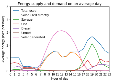
Here we can see that, on average, the solar generation in this system exceeds the demand during the middle of the day, resulting in the total energy used by the community being almost entirely satisfied by solar energy. In the evening, when the load demanded by the community increases and the solar generation decreases, the energy is instead supplied by a combination of battery storage, the grid network, and the diesel generator which continue to be used throughout the night.
It is important to note that the values shown here are for an “average” day and likely not reflective of any single day. Aside from the variations in solar generation and the load demanded, it is far more likely that in any given hour only one or two energy sources would be used at a time. By considering all of the days in the simulation we have artificially smoothed the data to present the averages.
Let’s instead look at the first day of data for the simulation period:
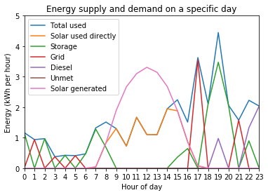
As we can see, the data is much spikier as it displays the variation between consecutive hours, rather than smoother averages. We can see how once again solar meets most of the demand during the day but during the evening and night the energy is supplied by either battery storage or, if available, the national grid - whose sporadic availability results in a seemingly peaked supply profile.
Electricity availability
We can also use the outputs of example_simulation_performance to
investigate the availability of different electricity services and the
times at which different energy sources are used, including the overall
measure of service availability recorded in the Blackouts variable.
Let’s once again consider an “average” day to visualise the availability:
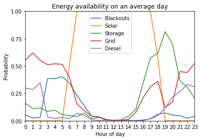
Here we can see that the blackout periods are not consistent throughout the day: although the average is 10% of the time they are much more frequent in the early morning, likely because the battery storage is depleted and the sun has not yet risen. As expected solar energy is always available (at least somewhat) during the day and never at night. Battery storage is used most of the time in the evening and more rarely throughout the night, when grid power is more commonly used. The diesel generator is also sometimes used during the evening and early hours of the morning, but rarely throughout the night.
Visualising seasonality
CLOVER allows us to investigate both the magnitude and timings of electricity supply and demand in the system at several different timescales. Given that the demand profiles and resource availability change throughout the year, it can be useful to visualise the variation at an annual timescale to identify any seasonal variation:
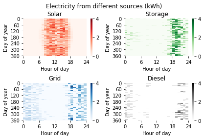
From this we can see that, as expected, solar energy provides most of the energy during the daytime but has periods of reduced supply in the third quarter of the year. Battery storage provides electricity mainly during the evening just after the sun goes down, with the time of sunset visibly later in the day during the middle of the year, whilst the grid provides power both during the evening and early hours of the morning. The diesel generator has a more seasonally varying profile: it is used less often in the summer months, when solar generation is higher and lasts for longer during the day, pushing back the times when storage is required and reducing the need for diesel generation.