Electricity generation

This section provides an overview of how to set up the electricity generation in CLOVER using its three modules solar, diesel and the national grid network. Further modules with new technologies could be added in the future to increase its functionality.

Solar

Preparation

The Solar module allows the user to get solar generation data for their location using the Renewables.ninja interface. Because this module relies on this external source of data it acts differently from other CLOVER modules, but ultimately returns the format of data that we expect from all of the generation files.

First, complete the “PV generation inputs” CSV file in the PV folder, which itself is located in the Generation folder. Let’s take a look at the inputs:

	0	1	2
0	tilt	29	degrees above horizontal
1	azim	180	degrees from north
2	lifetime	20	years

These should all be straightforward: we assume our panels are south-facing (180\(^{\circ}\) from North) and has a lifetime of 20 years, typical for a solar panel and used by CLOVER to account for module degradation. We also have stated that our panels will have a tilt (or elevation) of 29\(^{\circ}\) above the horizontal, or make a 29\(^{\circ}\) angle compared to flat ground (which would be 0\(^{\circ}\)). This angle could (for example) be the tilt of a roof that the panels are assumed to be located on, or it could be the optimum angle that maximises total energy generation over the course of a year (which can be found using the Renewables.ninja web interface, or many other programmes).

Getting solar generation

Our goal is to get 20 years of solar generation data for our location at an hourly resolution. The data will be the output energy of one functional unit of nominal power of the PV for each hour of the year, assuming it is installed at the specified location and orientation. The functional unit of nominal power (also called the nameplate capacity) is the kilowatt-peak (kWp), defined to be instantaneous power output of a PV array under standard test conditions (1000 W/m\(^2\)). This value is most commonly reported when buying solar modules, for example a panel with a nominal power (or nameplate capacity) of 300 Wp (0.3 kWp) would provide 300 W of power when illuminated under standard test conditions, or have a higher output if the illumination were higher (and vice versa). The actual power received from a module of a given capacity depends on many factors, for example the amount of illumination on the panel and the losses from a variety of sources, but Renewables.ninja calculates these automatically for us.

Using this functional unit makes it easy to scale up the generation capacity to the desired amount in a simulated system. First, check that you have already updated the location and filepaths of the Solar module and run the script (using the green arrow in the Spyder console). Here we run it like so:

The Solar module contains several nested functions which automatically provide a step-by-step process to send data to Renewables.ninja about the system parameters, account for the orientation of the system, and return ready-to-use data. We want to get 20 years of solar data but unfortunately the archives do not go back that far, so instead we will get 10 years of data and repeat it: this will allow us to keep the year-on-year variation whilst also covering our entire desired time period.

To do this we run a function which gets one year of solar generation and repeat the process until we have 10 years. In the Bahraich example we have data from 2007 to 2016, so let’s replicate this. First we will generate the data for 2007 by running the following function:

This automatically saves a CSV file for us, and we can look at the first day’s worth of entries:

    Hour     kW
0      0  0.000
1      1  0.000
2      2  0.000
3      3  0.000
4      4  0.000
5      5  0.000
6      6  0.000
7      7  0.009
8      8  0.184
9      9  0.419
10    10  0.591
11    11  0.687
12    12  0.733
13    13  0.697
14    14  0.594
15    15  0.417
16    16  0.192
17    17  0.017
18    18  0.000
19    19  0.000
20    20  0.000
21    21  0.000
22    22  0.000
23    23  0.000

As expected, we start getting solar generation from 6:00 (note that Python begins counting from 0, so the hours of the day run from 0 to 23) which peaks in the middle of the day and finishes by 17:00.

We then run the same function for the following nine years:

Solar().save_solar_output(gen_year = 2008)
Solar().save_solar_output(gen_year = 2009)
...
Solar().save_solar_output(gen_year = 2016)

Until we have 10 years of data. Now we can compile the data together using a function that stitches the data together in order, from the starting year of 2007, then repeats it to give the full 20 years of generation data:

This file contains the total solar generation expected for the 1 kWp unit panel over the course of 20 years, which is what we aimed to achieve. This is the file that is imported in the Energy_System module and used to calculate the total PV generation in a system. Use this process to generate solar data for your location.

Extension and visualisation

For interest, let’s see its cumulative generation over its lifetime, rounded to the nearest kWh:

Cumulative generation: 36655.0 kWh
Average generation: 5.0 kWh per day

This panel is expected to produce 36.7 MWh of energy over its lifetime, or around 5.0 kWh of energy per day - this is reasonable given the location of the panel in a relatively sunny location in India.

We can quickly visualise its generation over the course of the first year of its lifetime by taking the first 8760 hours (24 hours times 365 days) and plotting this as a heatmap:

As we might expect, the solar output varies throughout the year with longer periods of generation during the summer months. Some days have far less generation, potentially due to cloudy conditions. We can also see the total daily generation over the course of the year by taking the sum of the reshaped solar_gen_year object and plotting the result:

Troubleshooting

The reason why we need to import the data from Renewables.ninja manually is because the API will flag multiple repeated requests to its servers and deny access. This makes it not possible to put the Solar().save_solar_output(gen_year) function into a for loop for convenience, as the code will be executed faster than that which the API will allow. This will also apply if you manually run the function too quickly, so if you receive an error message relating to the API then wait for around one minute and try again.

Periodically the Renewables.ninja changes its API settings which affects the way that the Solar module interacts with the website. This requires the CLOVER code to be updated, so if you identify this happening please email Philip Sandwell.

Grid

Preparation

The Grid module simulates the availability of the national grid network at the location, particularly when the grid is unreliable or has variable availability throughout the day. CLOVER assumes that when the grid is available it can provide an unlimited amount of power to satisfy the needs of the community for the entire hour in question or, if unavailable, no power can be drawn from it. The goal of the Grid module is to provide an hourly profile of whether the grid is available or not by using a user-specified availability profile (or several of them, if many are to be investigated).

First, complete the “Grid inputs” CSV file in the Grid folder, which itself is located in the Generation folder. Let’s take a look at the inputs:

    Name  none  all  daytime  eight_hours  bahraich
0      0     0    1        0         0.33      0.57
1      1     0    1        0         0.33      0.61
2      2     0    1        0         0.33      0.54
3      3     0    1        0         0.33      0.50
4      4     0    1        0         0.33      0.48
5      5     0    1        0         0.33      0.48
6      6     0    1        0         0.33      0.46
7      7     0    1        0         0.33      0.34
8      8     0    1        1         0.33      0.25
9      9     0    1        1         0.33      0.30
10    10     0    1        1         0.33      0.35
11    11     0    1        1         0.33      0.35
12    12     0    1        1         0.33      0.33
13    13     0    1        1         0.33      0.29
14    14     0    1        1         0.33      0.32
15    15     0    1        1         0.33      0.35
16    16     0    1        1         0.33      0.35
17    17     0    1        1         0.33      0.32
18    18     0    1        0         0.33      0.39
19    19     0    1        0         0.33      0.14
20    20     0    1        0         0.33      0.18
21    21     0    1        0         0.33      0.46
22    22     0    1        0         0.33      0.47
23    23     0    1        0         0.33      0.51

This file describes five grid availability profiles, with each of the values corresponding to the probability that the grid will be available in the hour of the day specified on the left. Taking the sum of those values will give the average number of hours per day that the grid will be available. The profiles we have here are:

• none has no grid availability at all throughout the day, equivalent to not being connected to the grid
• all has full grid availability at all times
• daytime has grid availability throughout the day (8:00 until 17:59) but never at night
• eight_hours will provide approximately eight hours of power, randomly available throughout the day
• bahraich is an example profile from data gathered from Bahraich district, where availability is higher in the early morning and late evening but lower during the daty and early evening.

You can add further grid profiles by adding additional columns in the CSV file; they can have any name and values for grid availability must be in the range 0-1 as they represent probabilities. Save this file before moving on.

Getting grid availability profiles

Our goal is to get 20 years of grid availability data at an hourly resolution, represented as 0s (grid is unavailable) and 1s (grid is available), for each of the grid profiles listed in Grid inputs.

First, check that you have already updated the location and filepaths of the Grid module and run the script (using the green arrow in the Spyder console). Here we run it like so:

The Grid module is quite straightforward as it uses a single function to take an input grid profile, repeats the probability profile over a 20 year period, uses binomial statistics to transsform them into a profile of 0s and 1s, and save this availability as a new output CSV file to use later. To do this for all of the grid profiles run the following function in your console:

Grid().get_lifetime_grid_status()

Once this function is completed your new grid profiles will appear in your Grid folder and be ready to use, with their file names corresponding to the name of the status given in the input file (e.g. eight_hours_grid_status.csv). Given the nature of the calculation, this function will take a while to complete. This is normal and fortunately this process needs to be completed only once: the same grid availability profiles can be used in each of your investigations for reproducibility.

Extension and visualisation

Let’s take a closer look the bahraich grid profile by seeing how many hours per day it is available on average:

9.34 hours per day

The bahraich profile gives an average of 9.34 hours of availability per day, relatively normal for that region of rural India but definitely has potential to be improved by installing a minigrid system. Now let’s plot the grid availability throughout the day

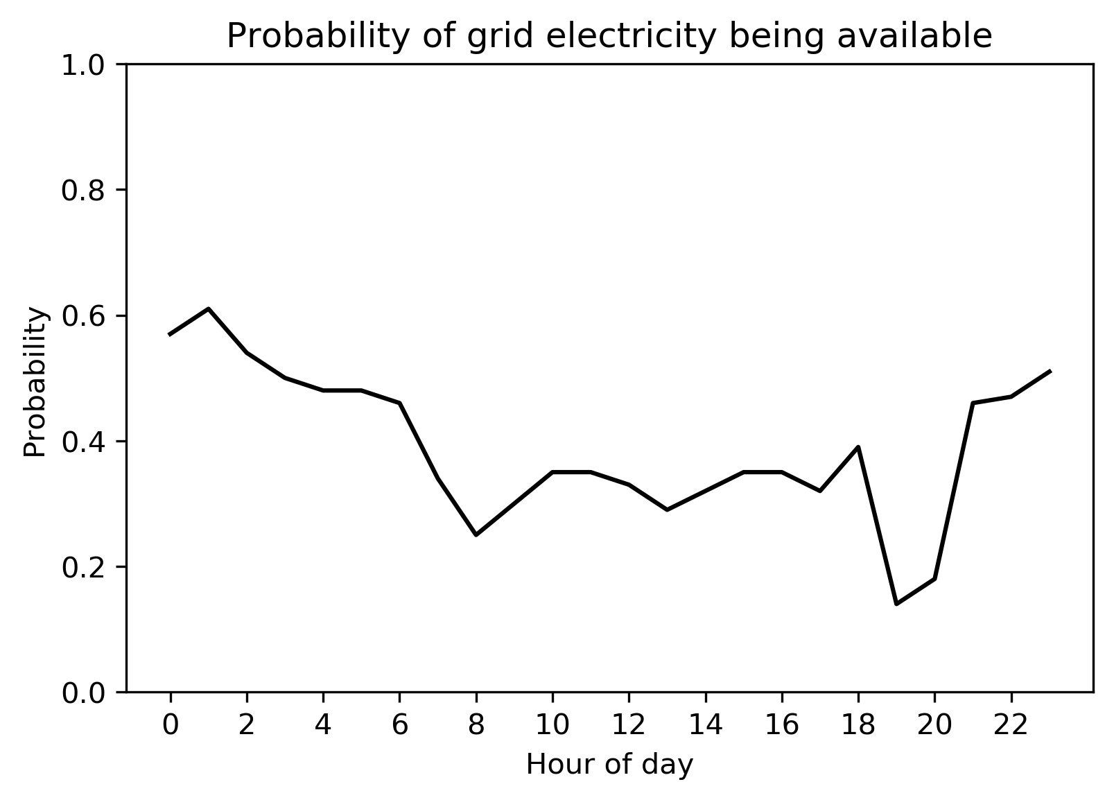
As we saw before, the grid is most likely to be available in the early morning and least likely to be available in the evening. We can also investigate the bahraich grid availability profile that we made using Grid().get_lifetime_grid_status(), for example by viewing whether the grid is available or not over the first year. Here we plot it using a colour scheme of white meaning the grid is available, or black when it is not (i.e. a blackout):

We can once again see the expected structure from the one-day availability input profile, but now with the randomness of day-to-day variations. There is greater availability in the mornings, but not always, and only on a very small number of days is power available between 19:00 and 21:00.

We can also compare the bahraich input profile to the synthesised availability profile to make sure they match up:

As we should expect, the output profile matches the input profile closely, but not exactly, owing to the random process that was used to generate it.

Troubleshooting

Rerunning the Grid().get_lifetime_grid_status() function will create new profiles: these will share the same statistics as a previously generated grid status but not be exactly the same. If you want to generate a new grid status but also want to keep ones you have already generated, it is recommended that you save your original files in another location and copy them back to the Grid folder once your new profile is complete.

CLOVER has the functionality to create grid profiles with variation throughout the day, but not throughout the year. If you want to include this, create an availability profile in a compatible format (20 years of hourly data, composed of 0s and 1s) using some other means, name it using the[name]_grid_status.csv format, and copy this CSV file to the Grid folder. CLOVER should be able to use this CSV file as an input later, the same as any others that it generates.

Diesel

Preparation

The Diesel module is a passive script, meaning that the user needs to provide it with inputs but not actively run any of its functions (CLOVER does this automatically instead). In the current release of CLOVER diesel generation is treated as a backup source of power when the other sources are unable to provide electricity, filling in periods of blackouts after a simulation is complete to provide greater levels of reliability. This means it can be used as a backup source of power in a hybrid system (for example switching on automatically when renewable generation is not sufficient) but not as dispatchable generation coming on at user-specified times. This functionality will be included in the next update of CLOVER.

First, complete the “Diesel inputs” CSV file in the Diesel folder, which itself is located in the Generation folder. Let’s take a look at the inputs:

    Diesel consumption   0.4    litres per kW capacity per hour
0  Diesel minimum load  0.35  Minimum capacity factor (0.0-1.0)

This input file contains just two variables but more parameters governing the usage of the diesel generator are included elsewhere. Diesel consumption refers to the hourly fuel consumption of the generator per kW of output, for example a generator providing 10 kW would use 4.0 litres of fuel per hour. CLOVER assumes that this fuel consumption is constant per kW of power being supplied, although in real systems diesel generators may have varying efficiencies dependent on the load factor.

Diesel minimum load is the lowest load factor that the generator is permitted to operate at (for example to avoid mechanical issues or degradation), expressed as a fraction. For example, a 5 kW generator would be forced to provide at least 1.75 kW (5.0 kW x 0.35) of power to ensure it runs above the minimum load factor even if the load were less than this, with the remaining energy being dumped.

Getting diesel generation

As mentioned above, as a passive script CLOVER uses the Diesel module automatically so the user does not need to run any of its functions. Nevertheless it is good practice to ensure that the script runs as expected, so check that you have already updated the location and filepaths of the Diesel module and run the script (using the green arrow in the Spyder console). Here we run it like so:

Now the script is ready to be used by the rest of CLOVER.